Cortex Tissue Mapping

Mapping diffusion measures (DTI, NODDI) to gray- and white-matter boundary surface.

This page demonstrates a recommended pipeline for mapping diffusion measures (DTI, NODDI) to the gray- and white-matter boundary following methodologies introduced by Fukutomi et al (2018) on brainlife.io. The goal of this tutorial is to show you how to process anatomical and diffusion data to generate anatomical warp fields, map microstructural measures to both the dMRI volume and the gray- and white-matter boundary surface. This tutorial will use a variety of brainlife.io applications to preprocess anatomical images and generate warp fields to a common template, preprocess dMRI data, map microstructural measures to the dMRI data, and map these measures to the gray- and white-matter boundary surface.

This tutorial will use a combination of skills developed in the Introduction tutorial, the Anatomical Preprocessing tutorial, and the Diffusion MRI Preprocessing tutorial you recently completed. If you haven't read our introduction to brainlife, or if you're not comfortable staging, processing, archiving, and viewing data on brainlife.io, please go back through those tutorials before beginning this one.

1. Anatomical preprocessing.

The first step of mapping microstructural measures to the gray- and white-matter boundary often involves processing the anatomical images. Anatomical (T1w) images, like all MRI images, require preprocessing to remove artifacts and align in a way that makes co-registration between functional or diffusion volumes and the anatomical image. In order to ensure anatomical fidelity in functional or diffusion analyses, it is imperative that anatomical (T1w) images and diffusion MRI images are aligned. One way we can make this easier for diffusion preprocessing applications like MRTrix3 Preprocessing is by aligning the anatomical images in such a way that the center of the brain is centered in the image. We refer to this as ACPC-aligned, as we are aligning the data to the anterior commissure-posterior comissure plane. In group analyses of anatomical properties, it is often helpful to register the anatomical (T1w) image to a common template, such as the MNI template. During this registration, fields known as warp and inverse warp are generated. These fields describe how to warp the anatomical (T1w) image to the common template (i.e. warp), or the common template to the anatomical image (i.e. inverse warp). These fields can then be used to generate any anatomical structure, including surfaces, derived from the anatomical (T1w) image. This is the first step in mapping diffusion measures to the gray- and white-matter boundary, and it is typically done with the FSL ANAT (T1) app. We will then need to generate cortical and white matter surfaces and brain region parcellations using Freesurfer. Surfaces from Freesurfer will be used to generate the final surface onto which diffusion measures will be mapped. Once we've processed our anatomical image, we can move on to diffusion MRI preprocessing.

2. Diffusion preprocessing

The next step in diffusion preprocessing is to actually preprocess the diffusion data. dMRI data, like any other MRI dataset, is quite noisy. Just like fMRI, dMRI data is sensitive to susceptibility distortions. This is when regions of the brain look "wavy" or fold inward or outward on itself in images. This is due to how the scanner sweeps across the entire brain during acquisition. Also, dMRI data is very susceptible to motion. Because some scans take a long time, it is nearly impossible for a participant to lie completely motionless. Even the most subtle movements can alter the results in a specific region and make your data less accurate. Finally, movement of the magnetic gradients can induce electromagnetic currents which can affect the measurement in any given location. These electromagnetic currents are called eddy currents, and they are due to the fact that electricity and magnetism are part of the same field, otherwise known as an electromagnetic field. Thankfully, we can use brainlife.io to correct for all of these common artifacts using MRTrix3 Preprocessing.

In addition to these artifacts, dMRI has very low signal-to-noise ratio (SNR), which directly impacts how well you can fit microstructural models and analyze diffusion data. This means that in any given location, the amount of diffusion signal is very low compared to the "noise" of the scanner. There are methods to lower the amount of noise across the brain, and thus increase the SNR. MRTrix3 Preprocessing has the capability to identify and remove noise using principal components analysis (PCA) and Rician analysis.

On top of these issues, dMRI data is sensitive to other artifacts and non-regularities, including gibbs ringing and bias field inhomogeneities, which can affect the quality of the data and how well measures can be derived from the data. MRTrix3 Preprocessing can deal with all of these issues for us!

Finally, once the dMRI data is preprocessed and cleaned, MRTrix3 Preprocessing will align the dMRI data to the anatomical data. This will ensure that any analyses we do with the dMRI data will be anatomically-informed and biologically-relevant.

Useful information about the preprocessing pipeline that MRTrix3 Preprocessing is designed to run -- Diffusion Parameter EStimation with Gibbs and NoisE Removal (DESIGNER) -- can be found in this original Neuroimage paper.

3. Diffusion modeling.

Once the dMRI data has been cleaned and aligned to the anatomical (T1w) image, the next step is to start fitting diffusion-based models to the data. The first, and most widely-reported model, is the Diffusion Tensor (DTI) model, which attempts to model how much and in what direction water moves in the brain using a tensor. Regions in which water is moving anisotropically, or in the same direction, will have a tensor that is very cigar-shaped. Regions in which water is moving isotropically, or equally in all directions, will have a spherical-shaped tensor. This model outputs four different measurements: axial diffusivity (how strong water movement is in the primary direction of movement); radial diffusivity (how strong water movement is in the non-primary directions of movement); mean diffusivity (how strong water movement is in any direction); and fractional anisotropy (how strong water movement is and how directional that movement is). Fractional anisotropy (FA) and mean diffusivity (MD) are the most widely reported measures. These measures can be used for group analyses and in tractography/tractometry pipelines, along with cortical white matter mapping pipelines. For this tutorial, we will use FSL DTIFit to fit the DTI model to our preprocessed data.

In addition to the DTI model, other models exist that can measure different properties of myelinated tissue. For example, the DTI model has a few fundamental limitations that do not allow it to fully measure diffusion-related processes. These include the inability to accurately measure regions of crossing fibers and high susceptibility to partial-voluming effects. Some models attempt to get around these limitation by extracting multiple components from the diffusion signal, including the anisotropic signal and the isotropic signal. This can be useful as each of these components of the diffusion signal come from regions with different tissue properties. This allows for a more precise measure of myelinated microstructural properties, especially in regions with crossing fibers and anatomical boundaries where large gradients in tissue properties exist. One of these models, the Neurite Orientation Dispersion Density Imaging (NODDI) model, was recently found to accurately measure myelinated tissue properties on the gray matter-white matter boundary. For this tutorial, we will use an accelerated application of this model NODDI Amico to map the NODDI model to our preprocessed data.

4. Microsturctural mapping to gray- and white-matter boundary.

Once our anatomical brain parcellations and microstructural maps are generated, the next step is to map the microstructural measures to a the gray- and white-matter boundary. Often, microstructural measures derived from diffusion MRI are only examined in white matter regions, as these measures are dependent on myelinated tissue. However, myelinated tissue does not stop right at the boundary between gray- and white-matter. Histological staining examinations have proven the existence of myelin into the cortex, especially at the boundary between the two tissues. Recent advancements in methodologies have addressed this hyperfocused approach by mapping myelin-related microstructural measures to the boundary between the gray- and white-matter Fukutomi et al (2018). These methods allow for a more thorough examination of the myelinated-related tissue properties of the brain.

To do this, the surface between the gray- and white-matter boundary must first be generated from the Freesurfer cortical (pial) and white matter surfaces. Following this, the microstructural measures are mapped to this surface following the methodologies implemented in Fukutomi et al (2018). On brainlife.io, we have adapted the methods into a brainlife app that generates the appropriate surfaces, warps to the common template (optional), and maps microstructural measures to the gray- and white-matter boundary.

More information on the the methodology can be found in this Neuroimage paper.

Now, let's get to work! The following steps of this tutorial will show you how to:

1. ACPC align the anatomical (T1w) image and generate the warp fields to the MNI template,
2. Generate Freesurfer Brain parcellation,
3. preprocess the dMRI data using MRTrix3 Preprocessing,
4. fit the DTI & NODDI models,
5. map measures to the gray- and white-matter boundary,
6. compute summary statistics of microstructural measures in cortical regions derived using Freesurfer (aparc.a2009s)

Copy appropriate data over from a single subject in the Tutorial data project

1. Click the following link to go to the project's page for the Tutorial
2. Click the 'Archive' tab at the top of the screen to go to the Archives page.
3. Select the following datatypes from one subject by clicking the boxes next to the data for subject 'test001':
   • dwi
     • Both dwi files (AP and PA dataset-tagged)
   • anat/t1w
   • anat/t2w
4. Click the 'Stage to process' button on the right side of the screen
   • For 'Project', select your project from the drop-down menu.
   • For 'Process,' select 'Create New Process' and title it "Network neuroscience - structural tutorial." Hit 'Submit.'
     • This will take you to the process on your Projects page
5. Archive the data in your project by clicking the 'Archive' button next to each dataset.

Your data should now be staged for processing and archived in your projects page! You're now ready to move onto the first step: preprocessing of the anatomical (T1w & T2w) images!

Preprocess anatomical (T1w & T2w) data using FSL

T1w data

1. On the 'Process' tab of your project, click 'Submit App' to submit a new application.
   • In the search bar, type 'FSL Anat (T1w).'
   • Click the app card.
2. On the 'Submit App' page, select the following:
   • For input, select the staged raw anatomical (T1w) image by clicking the drop-down menu and finding the appropriate datasets.
   • Select the boxes for 'crop' and 'reorient'. Leave all other defaults the same.
   • Select the box for 'Archive all output datasets when finished'
     • For 'Dataset Tags,' type and enter 'fsl_anat'
   • Hit 'Submit'
3. Once the app is finished running, view the results by clicking the 'eye' icon to the right of the dataset
   • Choose 'FSLeyes' as your viewer
     • This will load the the preprocessed T1w data.

T2w data

1. On the 'Process' tab of your project, click 'Submit App' to submit a new application.
   • In the search bar, type 'FSL Anat (T2w).'
   • Click the app card.
2. On the 'Submit App' page, select the following:
   • For input, select the staged raw anatomical (T2w) image by clicking the drop-down menu and finding the appropriate datasets.
   • Select the boxes for 'crop' and 'reorient'. Leave all other defaults the same.
   • Select the box for 'Archive all output datasets when finished'
     • For 'Dataset Tags,' type and enter 'fsl_anat'
   • Hit 'Submit'
3. Once the app is finished running, view the results by clicking the 'eye' icon to the right of the dataset
   • Choose 'FSLeyes' as your viewer
     • This will load the the preprocessed T2w data.

Once you're happy with the surfaces, you can move onto running Freesurfer!

Freesurfer

1. On the 'Process' tab of your project, click 'Submit App' to submit a new application.
   • In the search bar, type 'Freesurfer 7.1.1'
   • Click the app card.
2. On the 'Submit App' page, select the following:
   • For input, select the staged preprocessed, 'acpc_aligned'-tagged anatomical (T1w & T2w) images by clicking the drop-down menu and finding the appropriate datasets.
   • Select the boxes for 'hippocampal' and 'thalamicnuclei'. Leave all other defaults the same
   • Select the box for 'Archive all output datasets when finished'
     • For 'Dataset Tags,' type and enter 'fsl_anat'
   • Hit 'Submit'
3. Once the app is finished running, view the results by clicking the 'eye' icon to the right of the dataset
   • Choose 'freeview' as your viewer
     • This will load the following volumes and surfaces: aseg, brainmask, white matter mask, T1, left/right hemisphere pial (cortical), and white (white matter) surfaces.
   • To view the aparc.a2009s segmentation on an inflated surface, do the following:
     • Click File --> Load surface
       • Choose the lh.inflated and rh.inflated surfaces
       • Hit 'OK'
     • Select inflated surface of choice (i.e. left or right hemisphere)
     • Click the drop-down menu next to 'Annotation' and choose 'Load from file'
       • Choose the appropriate hemisphere aparc.a2009s.annot file (lh.aparc.a2009s.annot)
       • Hit 'OK'
       • The aparc.a2009s parcellation should be overlaid on your inflated surface! Now, repeat the process on the other hemisphere.

Once you're happy with the surfaces, you can move onto preprocessing your dMRI data!

Preprocess diffusion MRI data with MRTrix3 preproc.

1. On the 'Process' tab, click 'Submit App' to submit a new application.
   • In the search bar, type 'MRTrix3 preproc'
   • Click the app card.
2. On the 'Submit App' page, select the following:
   • For anat/t1w, select the staged ACPC-aligned anatomical (T1w) image by clicking the drop-down menu and finding the appropriate dataset.
   • For dwi, select the dwi image with the tag "PA" by clicking the drop-down menu and finding the appropriate dataset.
   • For dwi (reverse), select the dwi image with the tag "AP" by clicking the drop-down menu and finding the appropriate dataset.
   • for acqd, choose 'posterior -> anterior (y) (PA) by clicking the drop-down menu and finding the appropriate choice.
   • Leave all the other options as default
   • Select the box for 'Archive all output datasets when finished'
     • For 'Dataset Tags,' type and enter 'acpc_aligned'
   • Hit 'Submit'
3. Once the app is finished running, view the results by clicking the 'eye' icon to the right of the dataset
   • Choose 'fsleyes' as your viewer
   • Only have the file titled 'dwi.nii.gz' selected in the viewer
4. You can also generate a QA image of the DWI-T1 alignment by running the 'Generate images of DWI overlaid on T1' using the ACPC-aligned anatomical image and the preprocessed dMRI image generated above! Archive the results and save with the tag 'qa dmri-t1 overlay'.

Once you're happy with the results, you can move onto fitting the CSD, DTI, and performing tractography!

Fit the DTI & NODDI models.

DTI

1. On the 'Process' tab, click 'Submit App' to submit a new application.
   • In the search bar, type 'FSL DTIFIT'
   • Click the app card.
2. On the 'Submit App' page, select the following:
   • For dwi, select the preprocessed dMRI image generated above by clicking the drop-down menu and finding the appropriate dataset.
   • For shell, type '1000' to fit the model on the b=1000 shell
   • Select the boxes for 'kurtosis', 'sse', and 'multishell'
   • Select the box for 'Archive all output datasets when finished'
     • For 'Dataset Tags,' type and enter 'cortex'
   • Hit 'Submit'
3. Once the app is finished running, view the results by clicking the 'eye' icon to the right of the tensor dataset
   • Choose 'fsleyes' as your viewer
     • This will load the tensor images for inspection.
4. You can also generate a QA image of the tensor fits by running the 'Generate figures of tensors' using the tensor datatype generated above! Archive the results and save with the tag 'qa tensor'.

NODDI

1. On the 'Process' tab, click 'Submit App' to submit a new application.
   • In the search bar, type 'NODDI AMICO'
   • Click the app card.
2. On the 'Submit App' page, select the following:
   • For dwi, select the preprocessed dMRI image generated above by clicking the drop-down menu and finding the appropriate dataset.
   • For 'dPar', type '0.0011' to fit the model using the appropriate parallel diffusion rate in cortex
   • Leave all other options as default
   • Select the box for 'Archive all output datasets when finished'
     • For 'Dataset Tags,' type and enter 'cortex'
   • Hit 'Submit'
3. Once the app is finished running, view the results by clicking the 'eye' icon to the right of the tensor dataset
   • Choose 'fsleyes' as your viewer
     • This will load the NODDI images for inspection.
4. You can also generate a QA image of the noddi outputs by running the 'Generate figures of NODDI' using the NODDI datatype generated above! Archive the results and save with the tag 'qa noddi'.

If you're happy with the results, you're ready to move onto mapping microstructural measures to the gray- and white-matter boundary!

Map microstructural measures to the gray- and white-matter boundary.

1. On the 'Process' tab, click 'Submit App' to submit a new application.
   • In the search bar, type 'Cortex Tissue Mapping'
   • Click the app card.
2. On the 'Submit App' page, select the following:
   • For dwi, select the preprocessed dwi output generated above by clicking the drop-down menu and finding the appropriate dataset.
   • For freesurfer, select the Freesurfer output generated above by clicking the drop-down menu and finding the appropriate dataset.
   • For tensor, select the tensor output generated above by clicking the drop-down menu and finding the appropriate dataset.
   • For noddi, select the NODDI output generated above by clicking the drop-down menu and finding the appropriate dataset.
   • For warp, select the warp output generated above for the neuro/t1w datatype by clicking the drop-down menu and finding the appropriate dataset.
   • In the Advanced section, select the Freesurfer parcellation of choice by clicking the drop-down menu and finding the appropriate parcellation. For this tutorial, we will use the Destrieux Atlas (aparc.a2009s).
   • Leave all other options as defaults
   • Select the box for 'Archive all output datasets when finished'
     • For 'Dataset Tags,' type and enter 'noddi_dti_cortex'
   • Hit 'Submit'
3. Once the app is finished running, view the results by clicking the 'eye' icon to the right of the dataset
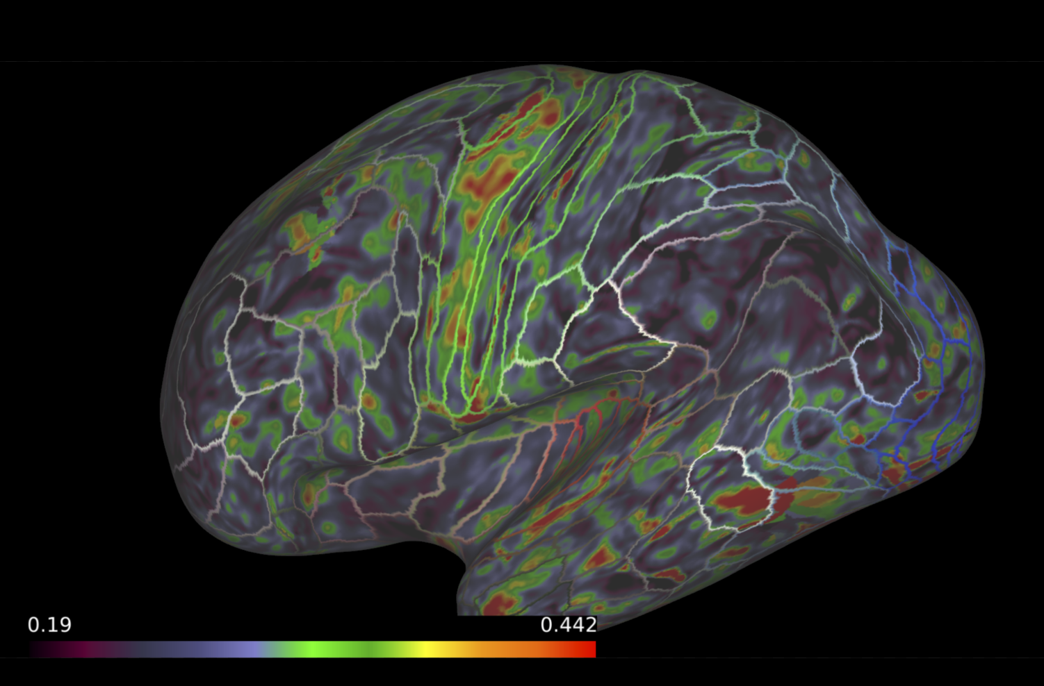
   • Choose the 'Connectome Workbench' viewer
     • This will load all the surfaces generated within the app and the microstructural measures.

If you're happy with the results, you're ready to move onto computing summary statistics in each region of the parcellation from Freesurfer!

Compute summary statistics.

1. On the 'Process' tab, click 'Submit App' to submit a new application.
   • In the search bar, type 'Compute summary statistics of diffusion measures mapped to cortical surface'
   • Click the app card.
2. On the 'Submit App' page, select the following:
   • For cortexmap, select the cortexmap output generated above by clicking the drop-down menu and finding the appropriate dataset.
   • Leave all other options as defaults
   • Select the box for 'Archive all output datasets when finished'
     • For 'Dataset Tags,' type and enter 'noddi_dti_cortex'
   • Hit 'Submit'
3. Once the app is finished running, view the results by clicking the 'eye' icon to the right of the dataset
   • Choose the 'File Viewer' viewer
     • You can then examine each summary statistic csv

Once you're happy with the results, you're finished with this tutorial!!